Selecting the Correct Tools for Inspection

Major items to be checked before introducing machine vision

Selecting the devices required for inspection

Choose the correct devices that meet the inspection requirements.

Camera / Controller / Lighting / Lens / Monitor
Sensing and judgment

Perform testing on the actual target.

Reference parts for OK and NG products
Inspection cycle time
Variety of inspection items
Selecting the installation location and procedure

Review the specific installation locations.

Target in motion/stationary
Environmental conditions, including ambient light and vibration
Controls for automation

Review the I/O controls.

Image capture timing / Judgment output / PLC control / Data output
On-site testing

Test on the actual production line.

Fine setup adjustment
Statistics
I/O control check
Understanding basic operations

Basic setup procedures to maintain stable inspection.

Setting tolerances / Sensitivity adjustment / Changing the inspection settings / Item registration

See product information on Intuitive Vision System

Detection judgment: determine whether the inspection is actually possible or not.

Preparation required for judgment

Prepare several samples of defective and non-defective workpieces.

To confirm the detectability with machine vision, it is effective to test it by using limit samples of defective and non-defective workpieces.

Preparing several types of limit samples will make the result closer to the result on an actual line.

Differentiation of MUST and WANT

For some inspections, you can set clear ranking for the detectability by differentiating MUST items that must be detected and WANT items that are preferably detected.

[ Non-defective workpiece ][ Defective workpiece(MUST) : Chipping / Burr / Deformation / White stain ][ Defective workpiece(WANT) : Chipping (small) / Burr (small) / Deformation (small) / White stain (small)]

When a specific quantitative difference is set between MUST and WANT, it is easier to judge the stability of detectability. For example, when you inspect a target with a size of 20 mm in the field view of 25 mm with a megapixel camera, one pixel measures 0.025 mm. On the assumption of one pixel as the minimum unit, the theoretical detection limit under this condition is 0.025 mm. In reality, however, there are various extraneous conditions so you need to allow some margin for the detection limit.

In the example above, when the depth of MUST-level chipping is 0.5 mm, it can be recognized as a change of 20 pixels and the detection is judged as possible. When the depth of a WANT-level chipping is 0.05 mm, it is a change of 2 pixels and the chipping can be assumed to be close to the detection limit.

MUST-level chipping: 0.5 mm → reliable detection

WANT-level chipping: 0.05 mm → detection limit

See product information on Intuitive Vision System

Download

Checking the judgment tolerance and margin

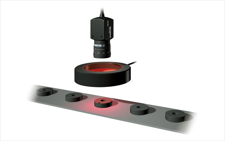
The reliable method to judge the detection stability is to check the statistical data of the values measured with multiple defective and non-defective workpieces. The graph shown below is the result of measuring 256 inspection targets with the statistical analysis function of the CV Series machine vision. Targets exceeding the upper limit line are detected as NG. The graph shows the level at which workpieces are detected as defective based on the upper limit setting.

When tolerance (upper limit) is set with sufficient margin

The average of the measured values is about 6.3. The red circles represent MUST-level defective workpieces and all of them well exceed the upper level.
The blue and green circles represent WANT-level defective workpieces. When the upper limit is set to 17.0, the workpieces in blue circles can be detected as NG.
Although the WANT-level defective workpieces in green circles cannot be detected with this setting, there is no chance that non-defective workpieces are detected incorrectly.

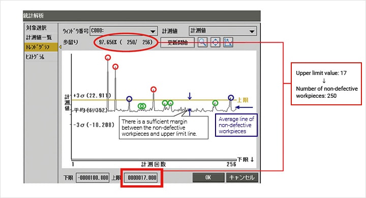
Upper limit value: 17 > Number of non-defective workpieces: 250

When the upper limit value is set more severely, from 17 down to 11, the number of non-defective workpieces reduces from 250 to 244, showing a reduction in yield rate.

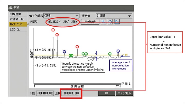
When severe tolerance is set to detect WANT-level defective workpieces as much as possible

The attempt to lower the upper limit further to detect green circles representing WANT-level defective workpieces may also detect non-defective workpieces as NG because the limit coincides with the maximum value of the fluctuation of non-defective workpieces.
This example shows that the defective workpieces in green circles are at the boundary with non-defective workpieces.

Upper limit value: 11 > Number of non-defective workpieces: 244

See product information on Intuitive Vision System

Download

Takt time and image processing time 1

Every time you use machine vision for inspection, you have to think about the processing speed of the system. The latest machine vision technology is capable of ultra high-speed processing and can inspect up to 100 targets per second depending on the inspection details. Note, however, that the image processing time varies greatly depending on the number of pixels of the camera, processing details, the number of processing items, etc. It is important to check the processing speed of the machine vision system and the takt time of the inspection line.

Machine vision processing flow

The following shows the flow of the inspection using machine vision.

[ Trigger input > Image capture/transmission > Image processing > Judgment output > Control ] [ Machine vision processing speed Image capture/transmission: several to several tens of ms/ Image processing: several to several hundreds of ms ] [ When converted into inspection cycle time Several hundreds to several thousands of targets/minute ]

See product information on Intuitive Vision System

Download

Takt time and image processing time 2

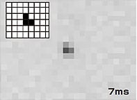
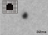
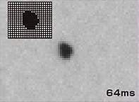
The minimum detectable resolution varies depending on the number of pixels of the camera used. As the number of pixels of the camera increases, the resolution also becomes higher, but the processing time increases as well. The following is an example of detection of black spots on a container when 0.31, 2, and 5 megapixel cameras are used. When the number of pixels in the binary images captured with these cameras are compared over the same field of view, there are great differences in the number of detecting pixels. This means that cameras with a higher number of pixels can provide more detailed detection. On the other hand, cameras with a higher number of pixels require longer processing time.

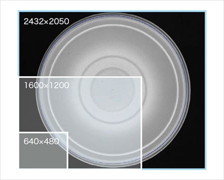
* The processing time and the number of pixels shown below are typical examples. The processing time is the shortest trigger interval.

3pixels

23pixels

55pixels