What Is a Reliability Growth Curve (Bug Curve)?

What Is a Reliability Growth Curve? Visualizing Software Quality with the Cumulative Number of Bugs

A reliability growth curve is a graph that shows the cumulative number of bugs detected over time as testing progresses. In the field, it is often referred to as a “bug curve.”

The structure of the graph is very simple. The horizontal axis represents the testing period (number of days tested or number of test cases executed), and the vertical axis represents the cumulative number of bugs detected. By plotting the total number of bugs found up to that point as testing progresses, the trend of bug detection becomes visible as a curve.

In many cases, a bug curve starts with many bugs being found, followed by a gradual slowdown in the detection pace, and eventually almost no bugs being found.

How to Read a Reliability Growth Curve | Determining Quality Status in the Initial, Middle, and Final Stages

The shape of the bug curve shows characteristic patterns depending on the stage of testing.

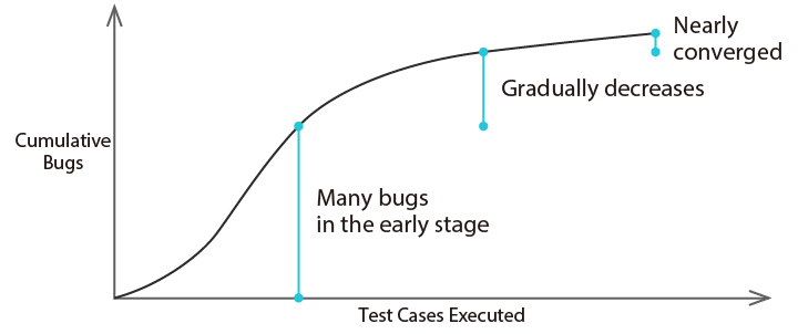
Initial Stage: Rapidly Increasing Phase

Immediately after testing begins, the number of bugs detected increases rapidly. On the graph, the curve rises sharply from the bottom left to the top right. This is because many relatively easy-to-find bugs remain. If almost no bugs are found at this stage, there may be a problem with the design of the test cases.

Middle Stage: Steady Increase Phase

As testing reaches the middle stage, the pace of bug detection becomes constant. On the graph, the slope of the curve becomes nearly constant, and the curve extends diagonally toward the top right. This is evidence that testing is progressing as planned.

Final Stage: Nearly Flat—The “Flattening Out” Phase

In the final stage of testing, the number of bugs detected decreases significantly, the rise of the graph slows down, and the curve becomes nearly horizontal. In the field, this state is described as “the curve is flattening out.” This means that almost no new bugs are being found, which is a sign that the software quality has stabilized.

An ideal bug curve starts from the bottom left, rises rapidly to the top right in the initial stage, shows a stable increase in the middle stage, and levels off in the final stage, forming a gentle S-curve.

• View PDF for details

Bug Curves Also Change with Changes in Testing

Bug curves do not always follow simple patterns like the one described above. Even after a curve has flattened out, the number of bugs often rises again when new types of tests are conducted.

For example, the bug curve of sensor control software for home appliances may take a shape like the one shown below.

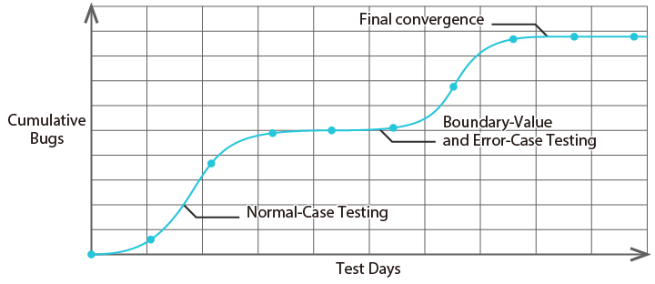
Home appliances such as air conditioners and washing machines need to process inputs from multiple sensors. Tests conducted when sensor values are within the normal range are completed early, but new bugs may be detected during testing of abnormal values or boundary values. Therefore, after the bug curve has nearly flattened out, it may rise again during boundary value testing or testing of abnormal operation. Ultimately, the curve becomes completely horizontal after all test perspectives have been covered.

How to Determine the Criteria for Release Approval

There are mainly two key points to keep in mind when using a bug curve to determine whether to approve a release.

Point 1: Is the latter half of the curve flat?

The most straightforward criterion is the “appearance of the graph.” Check whether the latter half (right side) of the curve is sufficiently close to horizontal and has stopped rising. For example, if a state where “about 0 to 2 bugs have been found in the past week” continues, you can judge that the curve has sufficiently leveled off.

Point 2: Is the estimated number of latent bugs within the acceptable range?

Another criterion is estimating “how many bugs still remain.” In practice, this involves using the number of bugs found in similar past projects as a reference to establish a benchmark for the expected number of bugs, then checking whether the number found is approaching that benchmark.

• View PDF for details

Checkpoints When No Bugs Are Found

If bugs are not found as expected, there are several typical causes.

Checkpoint 1: Is the test scope too narrow?

If bugs are hard to find, or if the graph is close to horizontal from the beginning, the scope of testing may be too narrow. This includes cases where only normal-case tests are conducted and abnormal cases are not tested, or where only specific functions are tested intensively. The solution is to review the test design document and check whether all functions and conditions are covered.

Checkpoint 2: Are you repeating the same tests over and over?

This may be because you are only executing similar test cases and are not testing from different perspectives. Conduct tests from various perspectives, such as long-run tests, load tests, and boundary value tests, in addition to functional tests.

Also, testers have their own habits. Changing the person conducting the tests can sometimes make it easier to find bugs.

Checkpoint 3: Are there any missed logs or records?

If you do not record all the bugs found, or if you confuse fixed bugs with unfixed ones, an accurate curve cannot be drawn. It is an ironclad rule to record all bugs, no matter how small. Make it a habit to check the records at the end of each day’s testing.

Checkpoint 4: Is bug fixing not keeping up?

It is possible that bug fixing is not keeping up with the pace of bug discovery. We recommend tracking not only the “cumulative number of discovered bugs” but also the trend of the “number of unfixed bugs” in a separate graph. If a bug found in a certain function is not fixed, it may not be possible to correctly test other operations of that function. This is called “blocking.” If blocking occurs, test progress may not go as planned, so it may be necessary to communicate with those responsible for fixing bugs to resolve the blocking early.

Checkpoint 5: Is the quality of the test cases sufficient?

If bug discovery levels off early and you feel anxious, there may be a problem with the quality of the test cases themselves. It is important to have experienced senior engineers review your test cases to improve your test design skills. Based on past experience, it is also important to conduct tests that target areas where bugs are likely to occur, that is, areas where it is difficult to ensure software quality.

Summary

The reliability growth curve (bug curve) is a powerful tool for visually understanding test progress and quality levels. Although it is a simple graph, its shape can reveal a great deal of information.
In embedded software development, once a product is shipped, it is difficult to make corrections, so ensuring quality before release is extremely important. By correctly understanding and utilizing the bug curve, you can find one answer to the difficult question of “when should testing be finished?”

• View PDF for details